Basis of SLA’s
An SLA is an agreement on service availability, performance and responsiveness. In this paper, only the availability SLA part is addressed. When indicating SLA’s however in this document, we are talking about the Minimum time a service or component needs to be available, or the maximum time allowed to be down.
When calculating SLA’s, it is important to know if the SLA is a monthly or yearly based SLA. For example:
| SLA level | Monthly | Yearly |
| 99.9 | ~43m | ~8:45hrs |
| 99.99 | ~4:20m | ~52:30hrs |
| 99.999 | ~26sec | ~5min |
In short, when targeting 99.99% uptime monthly, the service may only have a downtime of ~minutes in a single month with a maximum of 12x that time per year. If the SLA is yearly, the service could run for 11 months without a hiccup but would still fall in the SLA if unavailable for over 2 days in the last month.
How to achieve higher SLA
Given an SLA is an agreement between supplier and receiver of a service, it is up to the supplier to determine how that SLA is met, and in the agreement it is determined what the penalties are for not meeting the agreed SLA levels. How the supplier reaches that SLA is up to him as he weighs the cost of implementing redundancies against the risk of having to pay the penalties.
But while the SLA is a formal agreement, this document goes into the architecture to achieve a (higher) SLA level through the architecture of the services and applications.
Architectures
Applications run on infrastructure for which there is a risk that it might fail. The failure could be software related, power interruption, network related or even an unintended shutdown of a complete datacenter. There are many factors that can trigger a service to become unavailable. These factors can be represented in a percentage of possible failure.
For example, a single server might have a risk of being down for an x number of minutes which correlates to 0.5% of its planned uptime during a month or year (see above). That means the availability of that server should be 99.5% (which we call Uptime %)
To reduce the risk of a failure servers (services) are deployed in a Highly Available architecture. Generally, there are two main architectures available: duplicating a service (active/active) or having a master/slave configuration (active/passive). Obviously, there can be many copies or master/slave(s) to further reduce the risk of downtime.
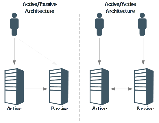
The architectures above show the high-level usage of High-Availability architectures. On the left is an active passive service. If the Active server fails, the passive server becomes active and can continue serving users. The downtime in the service is the failover time to switch the passive node to an active node and redirecting the user to that server.
On the right side of the figure is an active-active scenario. Users (in this case 2) are separated over two servers that are actively serving content. If one of the servers goes down, the downtime of the service is only the time required to redirect the user to the active server.
Multi-Geo deployments
When looking at deploying multiple services, the impact to the uptime% becomes significant. For example, say there is a service that has an uptime of 99.99%. This would imply the risk of that service going down is 0.01%. When this application can be deployed on a second datacenter that also guarantees 99.99% and there are no dependencies towards each other, the risk of downtime now is multiplied (0.01% * 0.01% = 0.000001% (the risk of the service being down in both datacenters at the same time)). When looking at a deployment in 3 datacenters the potential risk to downtime becomes 0.0000000001%. But this calculation only applies if the application in every datacenter is not depending on the other locations, and if every location can handle the max
Dependencies in service levels
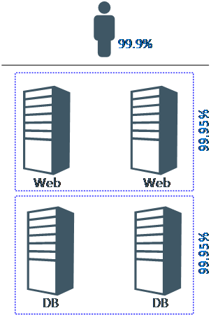
While the multi-geo calculations show a near 100% uptime can be provided, this is almost never the case and that is because of inter-dependencies. While a web-site can have an uptime of 99.95% it usually depends on a backend database for its functions. That database has an uptime as well, say 99.95%. The total uptime becomes 99.95% * 99.95% = 99.9%.
The more components are used in the dependency to make a service work for end-users or inter-related systems, the more impact this has on the uptime.
This calculation is because each component in the solution may sustain downtime to still achieve its uptime percentage. When that component is unavailable, which causes other components to be unavailable, the total amount of unavailable time increases. In short, the availability percentage is multiplied by the availability percentage of each component in case of a solution that is dependent on multiple components.
In the image above, each tier has a 99.95% uptime guarantee. This means that every tier may sustain a downtime of ~22 minutes per month. Given there are 2 tiers, the total downtime per month could go up to ~44 minutes, which equals to 99.9%.
Given complex systems are made up of a lot of components (power, cooling, storage, network, compute, OS, application), the impact to the uptime of these components must not be forgotten. Also, other dependencies such as data sources, connections into other systems and locations must be accounted for as well.
Conclusion
While the uptime SLA’s for services can be high, the total uptime (or equivalent risk of downtime) is highly impacted by the dependent service uptime SLA’s. While using redundant datacenters and redundant services help in increasing the uptime of a service, the desired uptime as indicated in the requirements ultimately drives the architecture. The architecture of a service will use the redundancy options to counterweigh the dependency loss of uptime.